I. Introduction

The East Sea of Korea is known to have many water masses which are identified by their physio-chemical properties such as temperature, salinity and dissolved oxygen.^[1]

Concerning the waves propagation related to ocean environments, there were some studies whose interests include polar front,^[2] mesoscale warm eddy,^[3,4] and bathymetry.^[5] There were also studies focused on sonar performances for decision aids of naval operations.^[6,7] All of these works, however, deal with the effects of single environmental factor on waves propagation or sonar performance in specific time and space.

This paper tries to examine the relations between water masses and sonar performances in the coastal region of Korea. The relations include the variations in temporal and spatial domains in the study area. The behaviors of acoustic waves in water are determined by sound speeds. Since, temperature is generally dominant factor determining sound speed, we consider temperature as key parameter for water mass analysis.

For measuring the performance of passive sonars, we usually consider maximum Detection Range (DR) under the environment and system parameters in operation. In shallow water, where sound waves inevitably interact with sea surface or bottom, detection generally maintains up to the maximum range. In deep water, however, sound waves may not interact with sea surface or/and bottom, and thus there may exist shadow zones where sound waves can hardly reach. In this situation, DR alone may not provide complete definition the performance of each sonar. For the sonar performances in deep water, in addition to the existing DR, we adopt another concept Robustness Of Detection (ROD). For the analysis of temporal and spatial variations of temperature, we use the database, Korean Ocean Temperature Model (KOTM) 3.0,^[8,9] which has 5-days means at each depth and every 5’x5’ grid point around Korean peninsula. We employ the Empirical Orthogonal Function (EOF) scheme to get the temperature variations.

Assuming two types of underwater targets at 5 m and 100 m, we examine the relations among the three factors : temperature, DR, and ROD. As an example of (passive) sonar operation related to seasonal variations of temperature, we give the comparisons of detection performance in February and August assuming a target at 100 m.

II. Analysis methods

2.1 Robustness of Detection (ROD)

In measuring sonar performances, we can employ some sorts of concepts. The popular ones are ‘effective range’, ‘near-continuous range’ and ‘maximum Detection Range (DR)’.^[8] Among these, the concept ‘DR’ is generally considered to measure the long range detection including shadow and convergence zones.

We can calculate the DR at each grid point as following.

Here, Di and N are the maximum DR at the i-th bearing and its number equally divided in 360°. However, it may not provide complete definition to measure the performance of a sonar, particularly in deep water. It may not guarantee consistent detection when there exist shadow zones in horizontal and vertical directions.

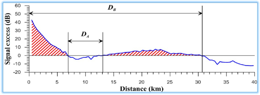
For complete description of sonar performance, we employ another definition ‘ROD’ as following.^[8]

Here, D_Aand D_B denote shadow range and maximum DR, respectively. Fig. 1 shows the definitions.

Fig. 1.

(Color available online) Shadow range (D_A) and maximum detection range (D_B).

2.2 Empirical Orthogonal Function (EOF)

In waters of less than 500 m, sound speed is mainly determined by temperature. Temperature variation may be analyzed using the EOF method. Spatio-temporal variations of temperature (T) may be decomposed into modal structure (A_n) and corresponding time coefficients (B_n) for each mode n as following.^[9]

Solving the eigen-value problems, we can get the reduced form of spatial variations,^[9]

where T,ei→,λi,Ndenote the temperature covariance matrix, eigen-vector, eigen-value and number of spatial points, respectively. T ^t represents the transpose of matrix T. The modal structure A_n is normalized to magnitude of standard deviation of B_nto have a physical unit °C, while B_n has not any physical unit. The fraction of i-th mode contribution to the total N modes of variation may be expressed as λi/∑i=1N(λi).

2.3 Temperatures/sound speeds

We use the temperature database, KOTM 3.0,^[8] which is the establishment of an average climatological marine environment data set for building up a sound exploration environment by re-analyzing the high resolution data around the Korean peninsula. The re-analyzed database was constructed by ensemble analysis over ocean numerical model results by verifying with observations from 1993 to 2018.^[9] The data set includes 5-days mean temperature, salinity and sound speed at each grid point of horizontal resolution 1/12° × 1/12°. At each grid, the data set gives non-linear depth resolution from the surface to the maximum depth of 6,000 m. From the data set, we select temperature or sound speed of every 10 m depth from the surface to 500 m in the study area.

The study area, about 200 km (longitude) × 200 km (latitude), has 82 grid points. At each point and every 10 m depth, we define the DR or ROD of each bearing, whose interval is 30°. Fig. 2 shows the 12 equal bearings of 30° interval with its DR (D_B). By averaging DRs or RODs over all bearings, we get the mean DR or ROD at each depth and point. Again, we normalize the mean DR to the maximum in all depths and points to get relative values in ratio.

Fig. 2.

(color available online) schematic diagram showing the maximum detection ranges (D_B) of 12 bearing angles at each point and depth.

2.4 Propagation model

We use an acoustic model based on the Gaussian beam tracing scheme^[10] to get acoustic fields (propagation loss) for 12 bearings at each depth and grid point. Since we consider the performance of passive sonars of mid-frequency, each depth of a grid point is the source position. From the propagation loss, we can compute DR or ROD by employing proper environment or system parameters such as noise level, directivity index, detection threshold etc. Since we are to examine the relations between water masses and sonar performances, we select the same parameters except propagation loss. In calculating propagation loss, we assume the same geoacoustic characteristics in the sediment layer at all grid points so that the propagation loss only reflects temperature or sound speed effect.

III. Analysis Results

3.1 Water mass vs. Sonar performance

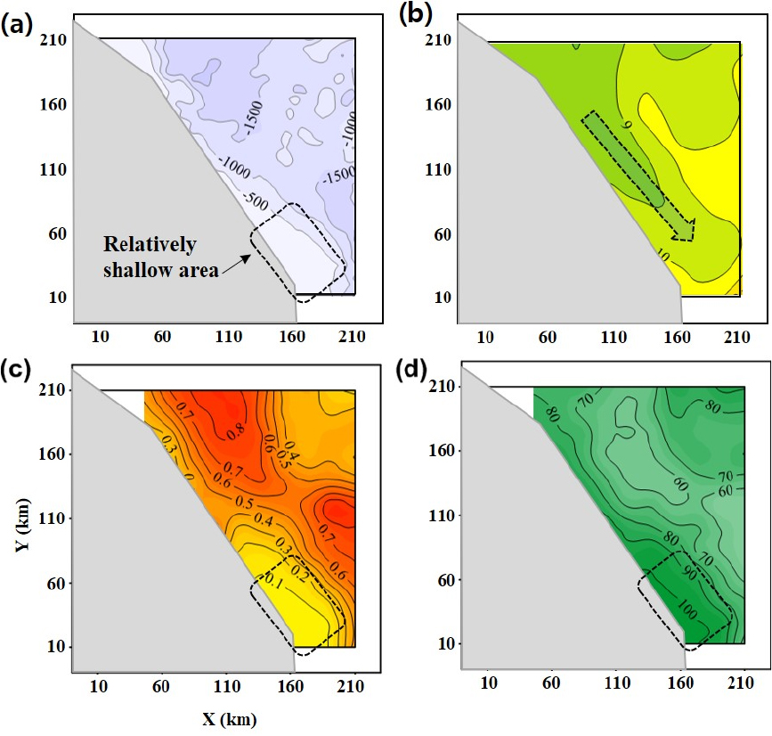
We give an example showing the relation between the DR and ROD, as defined in the section 2.1. Fig. 3 presents horizontal distributions of water depth (a), temperature (b), DR (c), and ROD (d). The temperature distribution comes from the data set re-analyzed at October 28, 2008. Depth distribution [Fig. 3(a)] shows that most of the area is actually deeper than 1,000 m, specially in northwestern and southeastern regions, except the coastal regions. The marked area in the southern part is regarded as continental shelf. Temperature distribution at 50 m [Fig. 3(b)] shows that cold water North Korean Cold Currents (NKCC) flows along the coast while warm water East Korean Warm Currents (EKWC) exist off the coast as shown in black and red arrows, respectively. The warm water is considered as related with meso-scale phenomena such as eddies and thermal fronts. Using the water depth and temperature data set as environmental input to the acoustic model, we calculate the DR and ROD assuming the source and receiver depth to be 50 m. Fig. 3(c) gives an example of DR in ratio relative to the maximum value calculated for all grid points and vertical depths considered. From the distribution, we can see that the ratios are relatively high in the northwestern and southeastern regions where depths are more than 1,500 m as in Fig. 3(a). On the other hand, in the regions of shallower depths (marked in broken line) and northern warm water [red arrow in Fig. 3(b)], we can see very low ratios. These low DRs may be caused by frequent bottom interactions of acoustic waves in the warm water region, leading large propagation loss. Another sonar performance, ROD [Fig. 3(d)] shows reverse patterns in general with that of DR. That is, the ROD gives low values in the deep regions in the northwest and southeast while high values in the regions of shallower depths (marked in broken line) and northern warm water [red arrow in Fig. 3(b)].

Fig. 3.

Horizontal variations of environment and sonar performance. (a) water depth, (b) temperature (50 m, October 28, 2008), (c) DR (SD/RD = 50/50 m), (d) ROD (SD/RD = 50/50 m).

As an another example showing the relation between water mass and detection performance, we present the temperature variations of 5 m and 100 m from the data set re-analyzed at February 21, 2007, and the corresponding DRs at source/receiver combinations of 100/5 m and 100/100 m, respectively. The surface temperatures [Fig. 4(a)] shows that the cold waters appear along the coast from northwestern region while the warm waters do in most of the area. At 100 m depth distribution [Fig. 4(b)], we can see that the cold waters develop much farther to the south along the coast and to the east, occupying most of the area.

Fig. 4.

Horizontal variations of environment and sonar performance. (a) temperature (0 m, February 21, 2007), (b) temperature (100 m, February 21, 2007), (c) DR (SD/RD = 100/5 m), (d) DR (SD/RD = 100/100 m).

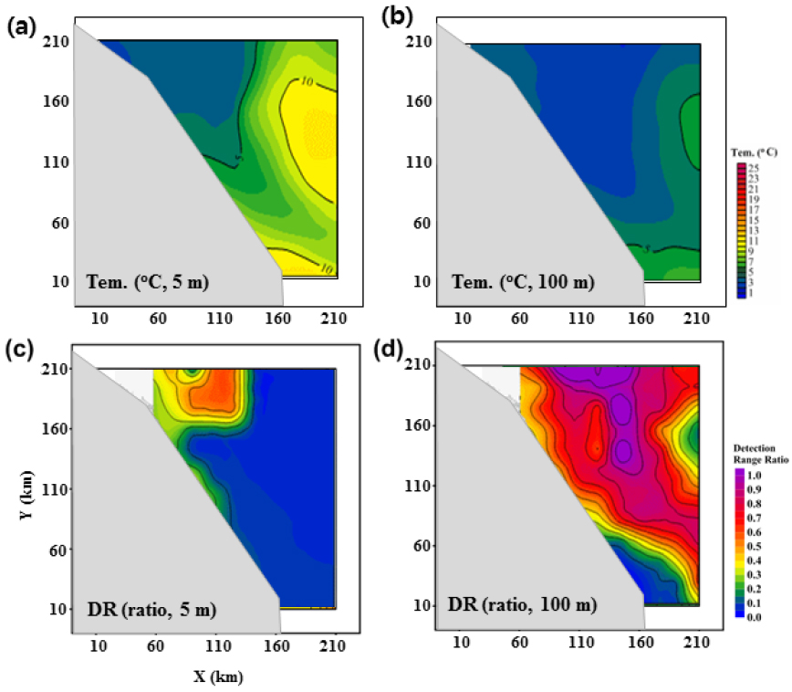
The corresponding DRs [Fig. 4(c), (d)] gives clear relations with the temperatures. That is, the DRs show high values in the area of cold waters but low values in the area of warm waters. We try analyses over other horizontal distributions of temperature, DR and ROD and find that the two facts are still valid; 1) Temperature (water mass) variations are closely related to DR and ROD, 2) DR and ROD have general reverse patterns.

Using Eq. (3) in section 2.2, we can calculate the spatial amplitudes {A_n(x,y,z)} and principal components {B_n(t)} for each mode n at each point. In order to examine the seasonal variation of each mode, we find the mean amplitude and mean principal component by averaging over the coordinate (x,y,z) at each time. Concerning the sonar performance, we assume two kinds of source located near the surface (5 m) and deep (100 m) while the two kinds of receivers to be at 100 m. The two receivers have different specifications so that they show different performance for the same environment and targets. Using these source and receiver configurations, we find the mean DR at each grid point as mentioned in section 2.3, and then find the total mean DR by averaging over all points at each time.

Fig. 5 shows the seasonal variations of modal amplitude multiplied by principal component (up) and sonar performances (down) where time step is 10 days. From the first two modes of temperature variations, we can see that mode1(‘’ symbols) follows typical patterns of seasonal variation while mode 2 (‘◆’ symbols) does not. We give the y-axis as reversed for the comparisons with the variations of sonar performance. Concerning the contribution to the total spatial variation in the study area, we estimate that the 1-st EOF mode accounts for 78 % and the 2-nd mode does 14 %.^[13] Mode 1 is regarded as representing typical seasonal variation of water masses both in surface (warm) and deep (cold) layers, while mode 2 representing the strength variation of surface mixed layer and the East Korean Warm Currents.^[13]

Fig. 5.

Seasonal variations of the first two modes (°C, up) and DR (ratio, down) (RD = 5/100 m, SD = 100 m).

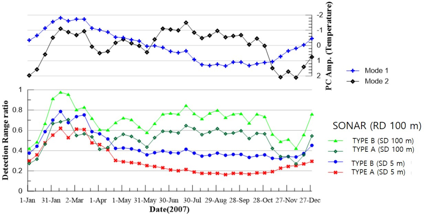
The sonar performance (Fig. 5, down), DR, which is averaged over all depths and grid points in the study area, gives seasonal variations for the four cases, two targets (located at 5 m and 100 m) and two receivers (different sonar types, located at 100 m). Comparing with the modal variations (Fig. 5, up), we can note that the DR for the surface target (source depth 5 m, ‘’ and ‘’ symbols) shows typical seasonal patterns and resembles the variations of mode 1 (‘’ symbols). The correlation coefficients between the variations of mode 1 and DR give very high negative values, –0.87 (Type A) and –0.94 (Type B). On the other side, we can see that the DR variation for the deep target (source depth 100 m, ‘’ and ‘’ symbols) shows similar patterns to the variations of mode 2 (‘◆’ symbols). The correlation coefficients between the variations of mode 2 and DR also give very high negative values, –0.89 (Type A) and –0.93 (Type B).

3.2 Water mass vs. Sonar operation

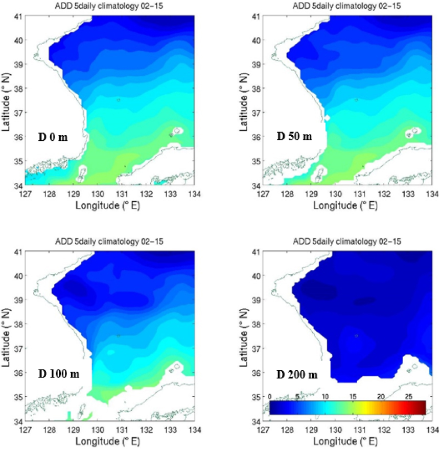
In this section, we give an example of sonar operation related to the water mass variation. In order to estimate the vertical limit of seasonal temperature variations, we review the horizontal distributions of some depths in the East Sea of Korea. We just presents the distributions in February and August representing one year variation. Fig. 6 gives the horizontal variations of mean temperature at 0 m, 50 m, 100 m, and 200 m in February. From the surface up to 100 m, the temperatures show very similar patterns implying the waters are well mixed by strong winds. The mean temperatures in August (Fig. 7), however, show very big changes in their variation patterns from the surface to 100 m. The distributions in February and August give somewhat similar patterns at 100 m and almost no noticeable differences at 200 m. This fact implies that most of seasonal variations occur from the surface to 100 m or more in the water column.

Fig. 6.

Mean temperature variations at selected depths (0 m, 50 m, 100 m, and 200 m) in February.

Fig. 7.

Mean temperature variations at selected depths (0 m, 50 m, 100 m, and 200 m) in August.

As an example of sonar operation related to seasonal variations of water mass, we try to compute sonar performance, DR, using the temperature data set depicted in Fig. 6 and Fig. 7.

We assume a target at 100 m, and the sonar (‘Type B’ in Fig. 5) located at 20 m (shallow) and 100 m (deep). Other parameters on the sonar and environment are same as in the previous section.

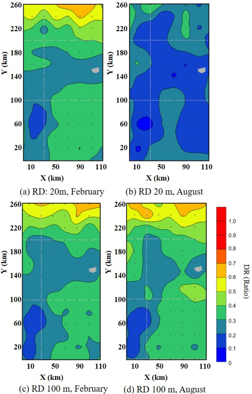
Fig. 8 shows the DR variations with the sonar depth varied between 20 m (shallow) and 100 m (deep) in February and August. For the details of performance variation, the smaller area, 110 km × 260 km, is selected from the larger one in Fig. 6 or Fig. 7. February and August are assumed to represent the winter and summer, respectively. When we keep the passive sonar at 20 m [Fig. 8(a), (b)], shallower depth, the DR shows very different patterns in February and August, being much poorer in August. When we change the sonar depth to be 100 m [Fig. 8(c), (d)], the DR shows very similar patterns in February and August. Moreover, the DR in February resembles the patterns at sonar depth 20 m in February such as in the northern region. That is, we can expect very similar and good performance of little seasonal variations when we locate passive sonars to deep enough (lower than 100 m).

Fig. 8.

Performance (DR) variations at the sonar depths 20 m (up) and 100 m (down) in February (left) and August (right).

IV. Conclusions

In the coastal region of the East Sea, the spatial variations of water masses have close relations with DR and ROD, where DR and ROD show general reverse patterns of variation. The EOF analysis over temperatures shows that the 1-st mode represents typical seasonal variation and the 2-nd mode represents strength variations of surface mixed layers and currents. The two modes are estimated to explain most of the variations (about 92 %). Assuming two types of targets located at 5 m (shallow) and 100 m (deep), the passive sonar performance (DR) gives high correlation coefficients about –0.9 with mode 1 and mode 2. Most of temporal variations of temperature occur from the surface up to 200 m in the water column so that when we assume a target at 100 m, we can expect detection performance of little seasonal variations with passive sonars below 100 m.