

I. Introduction
II. Finite Difference form of the Wave Equation for a Bowed String by a Digital Bow
III. Transmission Line based Bowed Sting Model
IV. Conclusions
I. Introduction
Helmholtz revealed that a bowed string consists of two straight-line segments at any instance joined by a sharply bent kink which travels along an apparent envelope of the vibration at the speed given by the fundamental frequency of the vibrating sting. At any location of the string, the velocity of the string alternates between two values whose ratio of the durations is the same as that of the distances from the location to each end. The frictional force is exerted on a bowing point by a bow through a stick and slip action which is synchronized with the movement of the kink.[1] After the Helmholtz’s pioneering works, the behavior of a bowed sting has been studied theoretically and experimentally. McIntyre et al.[2] announced a computer model for musical instruments covering woodwind, brass, and bowed string. Their model consists of an interconnection of non-linear elements such as a reed and a bow and linear elements such as a tube and a string. The model for a bowed string incorporated a mathematical form of the frictional bow-string force and the hysteresis rule, by which the pitch flattening is produced when the normal force exerted on the bowing point by a bow exceeds a critical value. Weinreich and Causse[3] used a digital bow, which senses the instantaneous velocity of a string at the imagined bowing point, and applies the calculated frictional force according to the measured velocity to the bowing point, in their experiments to get reproducible bowing conditions. Smith studied physical modeling using digital waveguides. The digital waveguide consists of two delay lines along which the sampled values of traveling waves propagate oppositely.[4] Giordano, Nakanishi and Pitteroff, Woodhouse developed numerical methods in which equations governing the behavior of a string were approximated to finite difference forms.[5], [6], [7]
A vibrating string has been analogized to an electrical transmission line in that both of them carry a traveling wave to one direction and a reflected wave from a boundary to the opposite direction resulting in a standing wave, which provides clues to explain the behaviors of them in their applied areas. In the analogy of a string to a transmission line, the displacement and the rigid end on the string had been analogized to the current and the open circuit on the transmission line, respectively.[8], [9], [10] However, it turned out that the displacement corresponds to the voltage and the rigid end to the short circuit through the theory of a transmission line and circuit simulations. Based on this discovery, the transmission line based plucked string model was built, and later integrated with the circuit for a sound box to make the circuit based classical guitar model.[11], [12] Also, the transmission line based struck string model was built by implementing the calculations for the hammer-string force in the well known finite difference form of the wave equation for a struck string into a circuit.[13] Now, a transmission line based bowed string model is proposed so that the ways of excitation of a string into motion using the analogy of a transmission line are completed. As in the transmission line based struck sting model, the calculation for the frictional bow-string force given by a digital bow is implemented into a circuit, and the calculated force in the form of the voltage is applied to a junction between transmission lines corresponding to a bowing point. The performance of the proposed model is demonstrated by showing that the velocity of the string at the bowing point from the proposed model is consistent with that from the finite difference form of the wave equation for a bowed string by the digital bow. The proposed model is built and simulated using PSpice.
The paper is organized as follow; the finite difference form of the wave equation for a bowed string by a digital bow is presented in section 2. In section 3, the transmission line based bowed string model is proposed, and the model output is compared with that from the finite difference form, and then conclusions are drawn in section 4.
II. Finite Difference form of the Wave Equation for a Bowed String by a Digital Bow
Giordano et al. announced the finite difference form of the wave equation for a bowed string assuming that a string element at the bowing point moves with the same velocity of a bow while sticking and allowing only a fixed frictional force for each of the sticking and the slipping states.[5] In this paper, the finite difference form is improved by adopting a digital bow which senses the instantaneous velocity of a string at the bowing point and exerts the calculated force for the measured velocity on the same point. The digital bow originally operated on a string with hardwares for a velocity sensing device and a force delivery apparatus, and now is implemented in software.
The frictional bow-string force exerted by a digital bow is formulated as
| $$F _{b} ( \nu _{r e l} )=F _{0} ( \nu _{r e l} / \nu _{0} )/[1+( \nu _{r e l} / \nu _{0} ) ^{2} ],$$ | (1) |
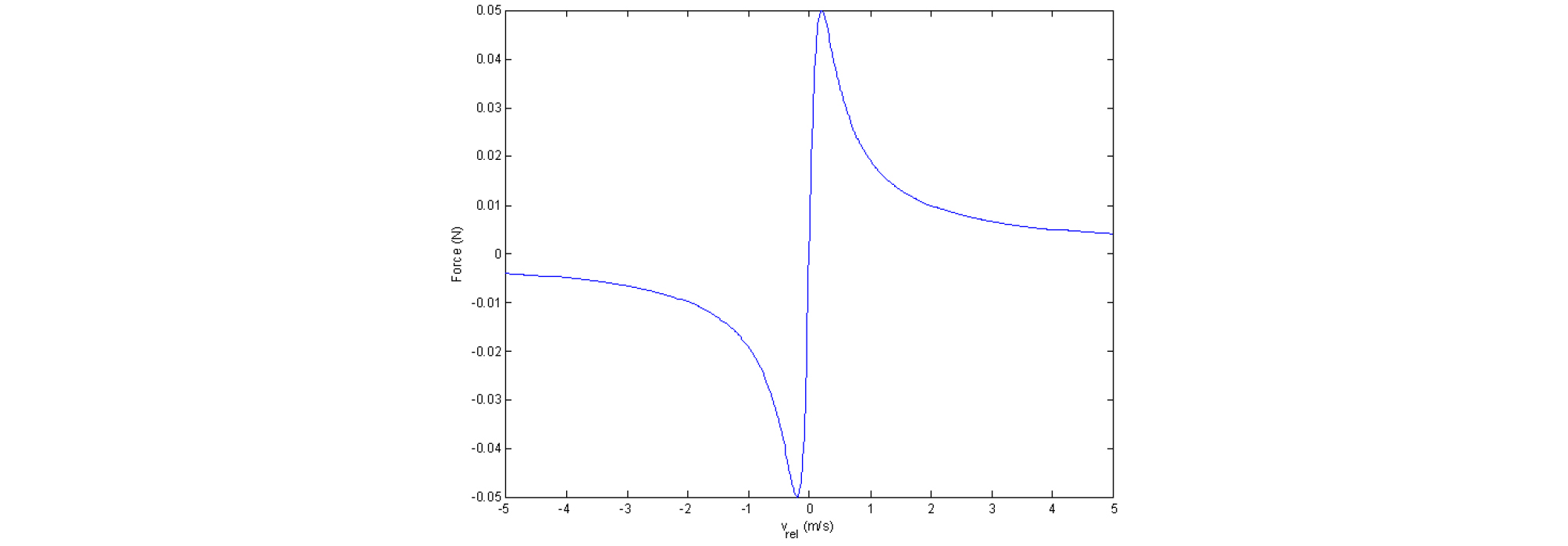
where , the relative velocity between a bow and a string, and is proportional to the normal force exerted on the bowing point by the bow, and determines the position of the maximum of the frictional bow-string force.[3] The frictional bow-string force used in the finite difference form is presented in Fig. 1. The values for and are set experimentally such that the velocity waveform at the bowing point represents a typical Helmholtz motion as will be shown.
The wave equation for an ideal flexible string with no damping is
| $$\frac{\partial^2y}{\partial t^2}=c^2\frac{\partial^2y}{\partial x^2},$$ | (2) |
where is the displacement of the string, and is the velocity of a wave on the string. is equal to where is the tension and is the mass per unit length. By sampling the Eq. (2) with a time step and a spatial step and then multiplying both sides by to make each of them the force exerted on an element of the string and finally adding the frictional bow-string force to the right hand side, the finite difference form of the wave equation for a bowed string is derived as
| $$\begin{array}{l}(\mu\triangle x)\frac{y(i,n+1)+y(i,n-1)-2y(i,n)}{(\triangle t)^2}\\\approx(\mu\triangle x)c^2\lbrack\frac{y(i+1,n)+y(i-1,n)-2y(i,n)}{(\triangle x)^2}\rbrack+F_b,\end{array}$$ | (3) |
where is a spatial index, and is a temporal one. The displacement at time step of can be derived from Eq. (3) as
| $$y(i,n+1)=2(1-r^2)y(i,n)-y(i,n-1)+r^2\lbrack y(i+1,n)+y(i-1,n)\rbrack+\frac{(\triangle t)^2}{\mu\triangle x}F_b,$$ | (4) |
where . At time step of , the bow-string force in Eq. (1) is calculated with the velocity of the string at the bowing point calculated at the previous time step. Then, the displacement at the bowing point and those at other locations are updated with the last term in the right hand side of Eq. (4) included and not included, respectively.[5] At the same time, the velocity of the string at the bowing point is updated as
| $$\nu _{s} ( n+1 ) = ( y ( i _{contact} ,n+1 ) -y ( i _{contact} ,n ) ) / \triangle t,$$ | (5) |
where is the bowing point.
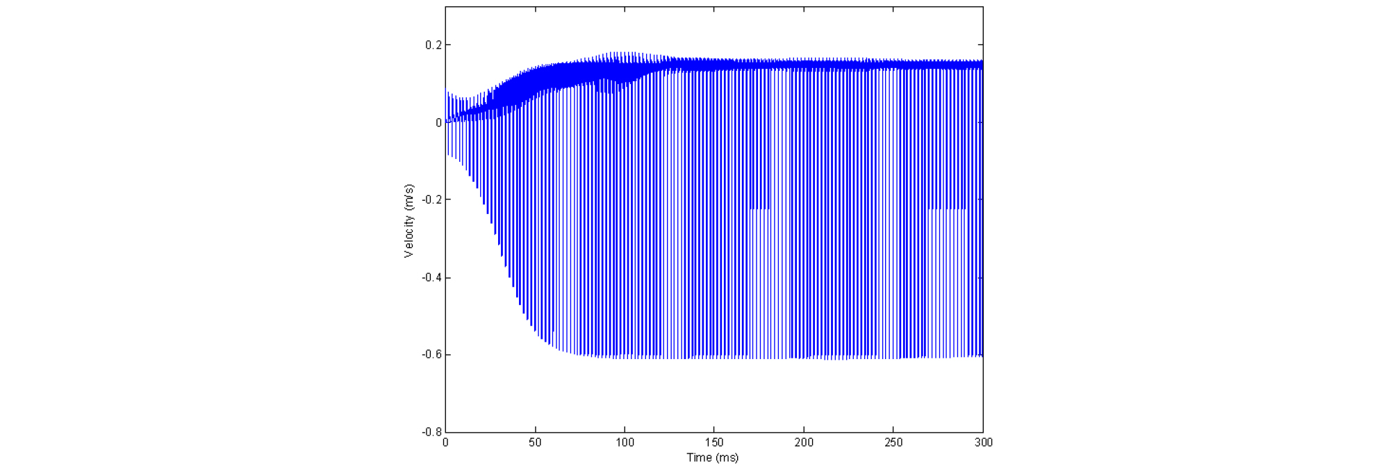
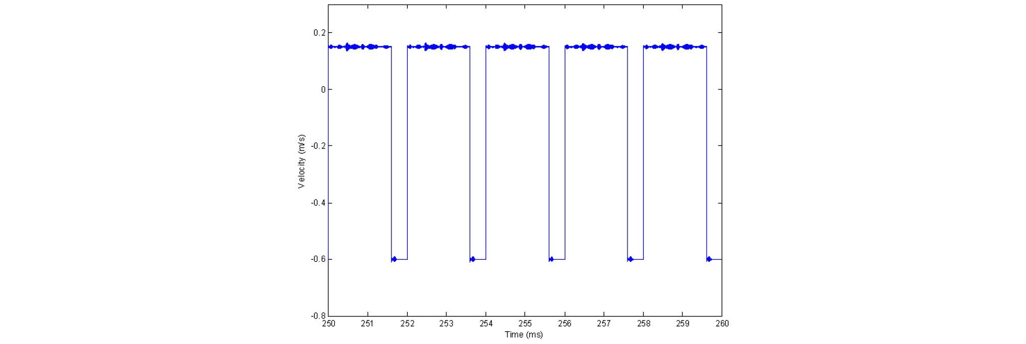
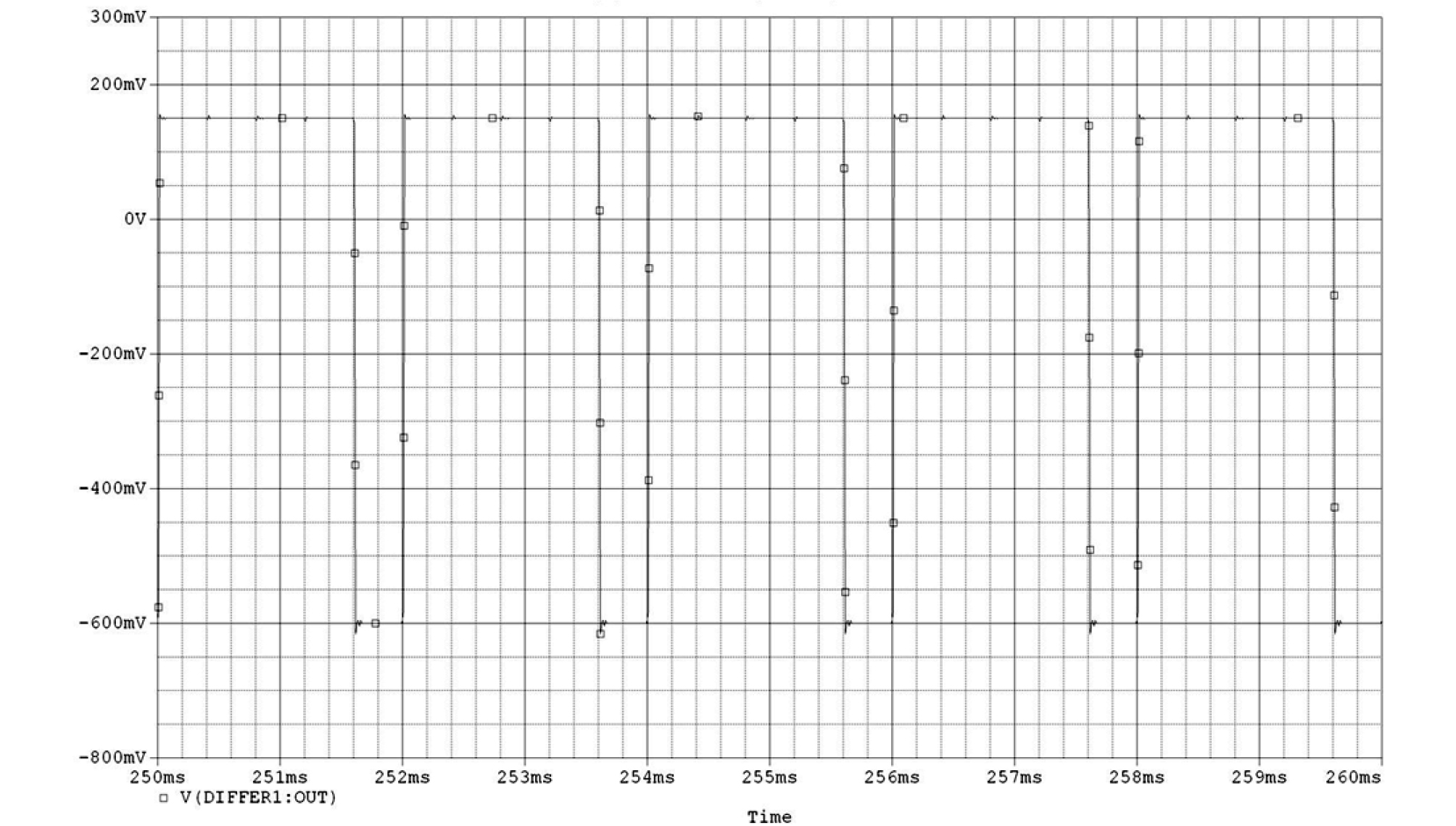
The velocity waveforms taken at the bowing point are presented in Figs. 2 and 3. The waveform in Fig. 3 is an enlarged portion of that in Fig. 2 from 250 ms to 260 ms which is a steady state of the velocity showing a typical Helmholtz motion of the string. The velocity of the string fluctuates about 0.15 m/s during sticking and about - 0.6 m/s during slipping, and the ratio of their durations is the same as that of the distances from the bowing point to each end. The finite value of the slope of the frictional force as shown in Fig. 1 from –0.2 m/s to 0.2 m/s, which pertains to the sticking state, gives rise to the difference of the velocity of the string at the bowing point from that of the bow during sticking.[3]
III. Transmission Line based Bowed Sting Model
The correspondences of the displacement and the rigid end on a string to the voltage and the short circuit on a transmission line and the implementation of the calculation for the frictional bow-string force into a circuit are applied to build a transmission line based bowed string model as shown in Fig. 4.

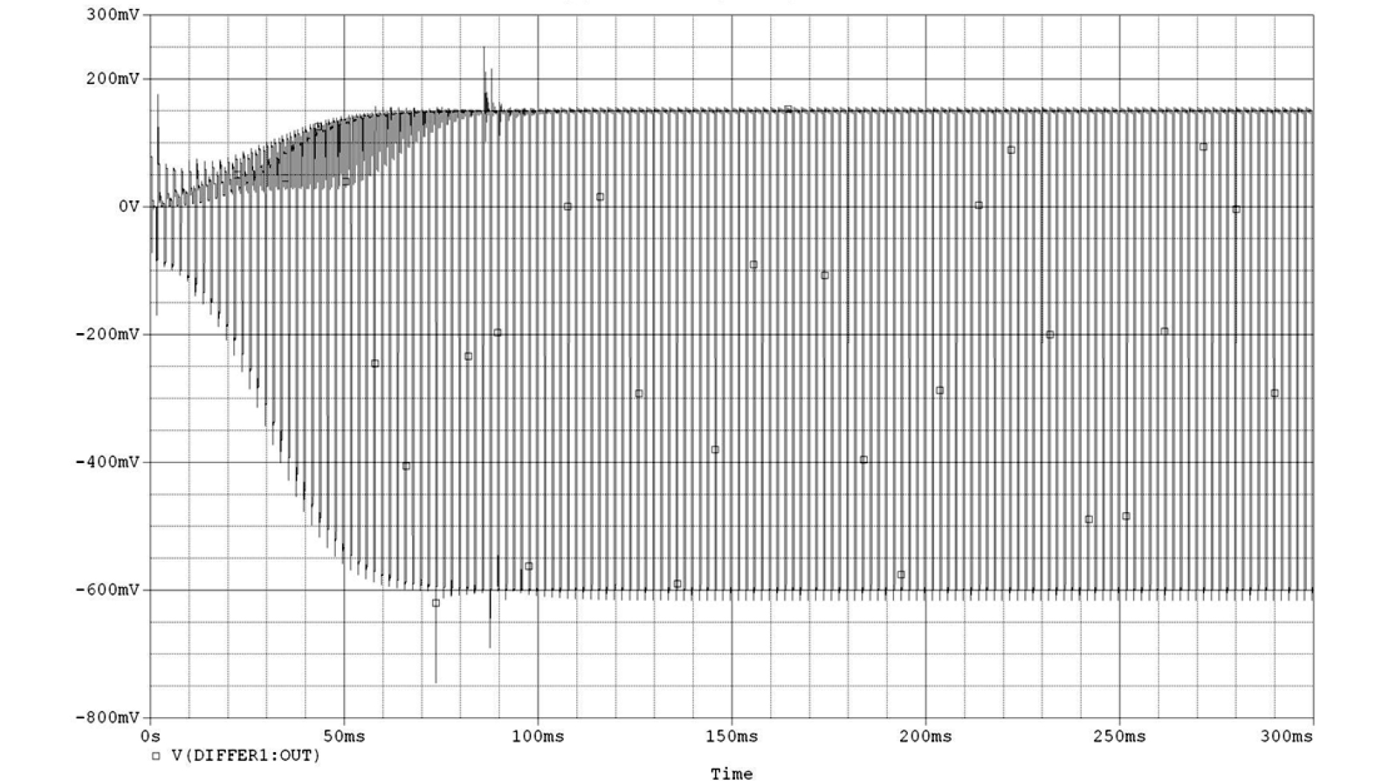
The time delays of the transmission lines, T1 and T2 are set to 0.2 ms and 0.8 ms, respectively, which corresponds to bowing a string at a distance one fifth from the left end of a string and the period as in the finite difference form. The characteristic impedances of the transmission lines are set to 1 kΩ arbitrarily. The voltage at the junction between the transmission lines is differentiated with respect to time with the differentiator with the gain of 1 to get the velocity of the string. The calculation for the frictional bow-string force given in Eq. (1) is implemented with a part provided by PSpice called Analog Behavioral Modeling (ABM1) taking the output of the differentiator as an input. The calculated force, that is, the output of ABM1, is delivered to the junction through the integrator with the initial value of 0 and the gain of 0.0035 and the voltage-controlled current source, G1. The integrator is used for the same reason as in the transmission line based struck string model. That is, the property that the displacement given by an applied force to a point of a string is maintained while propagating from the point to both directions is implemented with the integrator and its gain is set experimentally such that the resultant velocity is consistent with that from the finite difference form. The infinite output impedance of the voltage-controlled current source, G1 and the high input impedance of the voltage-controlled voltage source, E1 provide almost no loading at the junction, by which a wave on the transmission lines is not reflected at the junction. However, it is expected that some amount of a wave on a string is reflected at the bowing point due to the impedance mismatch between the string and bow hairs in real playing a string instrument. The voltage-controlled voltage source, E1 is used to avoid an oscillation that has nothing to do with the fundamental frequency given by the delay times of the transmission lines, T1 and T2. A direct connection between the junction and the input of the differentiator would result in the oscillation. The velocity waveforms taken at the output of the differentiator in Fig. 4 are shown in Figs. 5 and 6. The degree of a consistency between the velocity waveforms from the finite difference form in Fig. 2 and the proposed model in Fig. 5 is checked by calculating a correlation coefficient between them. The waveform from the proposed model is resampled to 500 kHz, which is the sampling frequency in the finite difference form, to calculate the correlation coefficient. The correlation coefficient is calculated to 0.9882, which demonstrates the high consistency of the proposed model with the finite difference form.
IV. Conclusions
The correspondences of the displacement and the rigid end on a string to the voltage and the short circuit on a transmission line and the implementation of the calculation for the bow-string force into a circuit are applied to build the transmission line based bowed string model. The performance of the proposed model is validated by showing that the velocity of the string at the bowing point from the proposed model is consistent with that from the finite difference form.
The proposed model does not account for the pitch flattening as in the existing model proposed by McIntyre et al. The adoption of the hysteresis rule associated with the pitch flattening in the proposed model would be nontrivial. However, the proposed model can be extended to a model for a bowed string instrument by connecting a circuit model for a body to the right end of the transmission line, T2 in Fig. 4. The circuit model for a body can be made by taking a modal test on a bridge of the body and fitting its calculated admittance to the measured one by the modal test. The circuit model for a body would provide controls of the resonances of the body and the synthesized sounds eventually. When it comes to the reflection of a wave at the bowing point, it has not been studied to the best knowledge of the author. A force delivery taking the reflection into account would improve the proposed model as in the transmission line based struck string model.
