

I. Introduction
II. Ship-radiated Noise Model
III. Network Architecture
3.1 Generator Architecture
3.2 Discriminator Architecture
3.3 Loss Function
IV. Results
4.1 Dataset
4.2 Spectral Feature Representation Analysis
4.3 Analysis
V. Conclusions
I. Introduction
Underwater data collection is a vital tool to solve many acoustic challenging tasks such as classification of different vessels[1] their velocities and location,[2] vessel tracking,[3] identifying targets and obstacles.[4,5] Generally, underwater data is collected with various measurement platforms integrated either on-board oceanographic vessels using sensor buoy system[6] or with the sonar arrays containing hydrophones.[7] Vast amount of recordings are made by military installations but that data is either incomplete or inaccessible to the acoustic researchers due to security reasons. This makes research groups record and collect data to create their own database of underwater sounds by installing their own equipment. Hence, the underwater data collection becomes a costly investment in human resources, time consumption and hardware equipment.
During the past few years, researchers are applying machine learning for the underwater acoustics.[1,4,8] However, underwater domain has an obvious shortage of the available data, which severely affects the accuracy of the applied ML techniques. To address this problem, the researchers, have been applying many data augmentation techniques in audio domain such as time stretching and scaling, pitch shifting on audio,[9,10] applying random frequency filters and interpolation of samples from input domain[11] to transform the existing data while preserving the input labels. In all these techniques, only pitch shifting and frequency filtering were effective to some extent while in other techniques; the network becomes invariant to these transformations.
Deep learning and more specifically Generative Adversarial Networks (GANs)[12] belong to the generative network family successfully used for generating realistic audio samples from the dataset provided for training.[13] For the audio generation, Long Short-Term Memory (LSTM) networks have also been used,[14] which generate audios with quite remarkable results but are notoriously slow in terms of computation due to their sequential processing. GANs are essentially useful for the data augmentation and expansion of the training dataset.[15,16] In this work, we propose to incorporate CycleGAN[17] (a variant of GAN) for the expansion of dataset by performing audio-to-audio translation to generate underwater ship radiated noisy engine sounds. The basic idea is to generate a new synthetic version of a given audios with a simple modification.
CycleGAN has been used widely for many applications including data augmentation and expansion.[18] In audio domain, it is deployed as voice conversion without parallel-data[19] and a front-end processor for the robust Automatic Speech Recognition (ASR) on perturbed utterances with emotion and voice quality.[20] CycleGAN- Voice Conversion (VC)[21] learns a sequence-based mapping function by incorporating CycleGAN with a gated Convolutional Neural Network (CNN)[22] and identity mapping loss.[23] CycleGAN consists of two GANs where one GAN takes the data from source domain (A) and translates the audios () to target domain (B), which are fed to the other GAN that translates back the input synthetic data () to the source domain (), hence the name CycleGAN. The key point is while the transformation it generates the synthetic data (), which belongs to the source domain (A) but not exactly (a) and hence a new synthetic data contributing to the expansion of database. To our knowledge, this work is the first effort to accommodate CycleGAN approach to work with the underwater audio synthesis.
To improve the data synthesis quality and the network performance, recently introduced components such as instance normalization,[24] dilated convolution[25] and interpolated convolution[26] produce promising effects on the results of image generation process[27] and audio generations as well.[22,25] There has been need for improvement in an overall end-to-end training network for the synthesized audios using these techniques. To satisfy this need, we proposed modified CycleGAN with improved generator, discriminator architecture and improved objective function. The contributions of this paper can be summarized as follows:
∙ Adoption of CycleGAN for performing the task of underwater ship engine sound transfer to another engine style.
∙ Usage of discriminator architecture based on PatchGAN in which dilated convolution increases the receptive field without increasing computation and memory costs while preserving the resolution.
∙ Improved generator architecture by using interpolated convolutions instead of up-sampling that mitigates the well-known checkerboard artifacts during up-sampling.
∙ An analysis of the performance of current sound synthesis technique on underwater ship engine data.
The content of the paper is organized as follows. In Section II, we present background of underwater ship radiated audio model. In Section III, we describe the proposed CycleGAN model by explaining improvement over original CycleGAN. In Section IV, we present the experimental results with analysis and comparison. At the end, we present a conclusion in Section V.
II. Ship-radiated Noise Model
Water sailing ship audios generally have three components: mechanical noise caused by the sailing ship, propeller noise by propeller cavitation, rotating sound and hydrodynamic noise by the irregular water flow.[28] The major constituents of ship-radiated noise are mechanical noise and propeller noise that can be seen as the addition of strong line spectrum and weak continuous spectrum as given in Eq. (1). Its energy is mainly distributed in low sound frequencies below 1000 Hz as shown in Fig. 1(a) and Fig. 1(b). Sources of underwater noise emissions in the environment have a bandwidth of 1 Hz to 100 KHz (a broad spectrum), which cover all existing frequencies as shown in Fig. 1(c).
| $$\mathrm x(\mathrm t)=X_l(\mathrm t)+\lbrack1+\mathrm a(\mathrm t)\rbrack X_c(\mathrm t),$$ | (1) |
where , a(t) and are time domain waveform of line spectrum component, periodic modulation and continuous spectrum component, respectively. Each term is a time-frequency atom (represented as a summation of sinusoidal and noisy components), which makes use of Inverse Fast Fourier Transform (IFFT) based efficient synthesis algorithms for the generation of the signal.[29] The Mel cepstrum (MCEP) is as good as conventional cepstrum and considered as an efficient parameter due to its relatively low order, making it a popular feature for underwater audio synthesis.
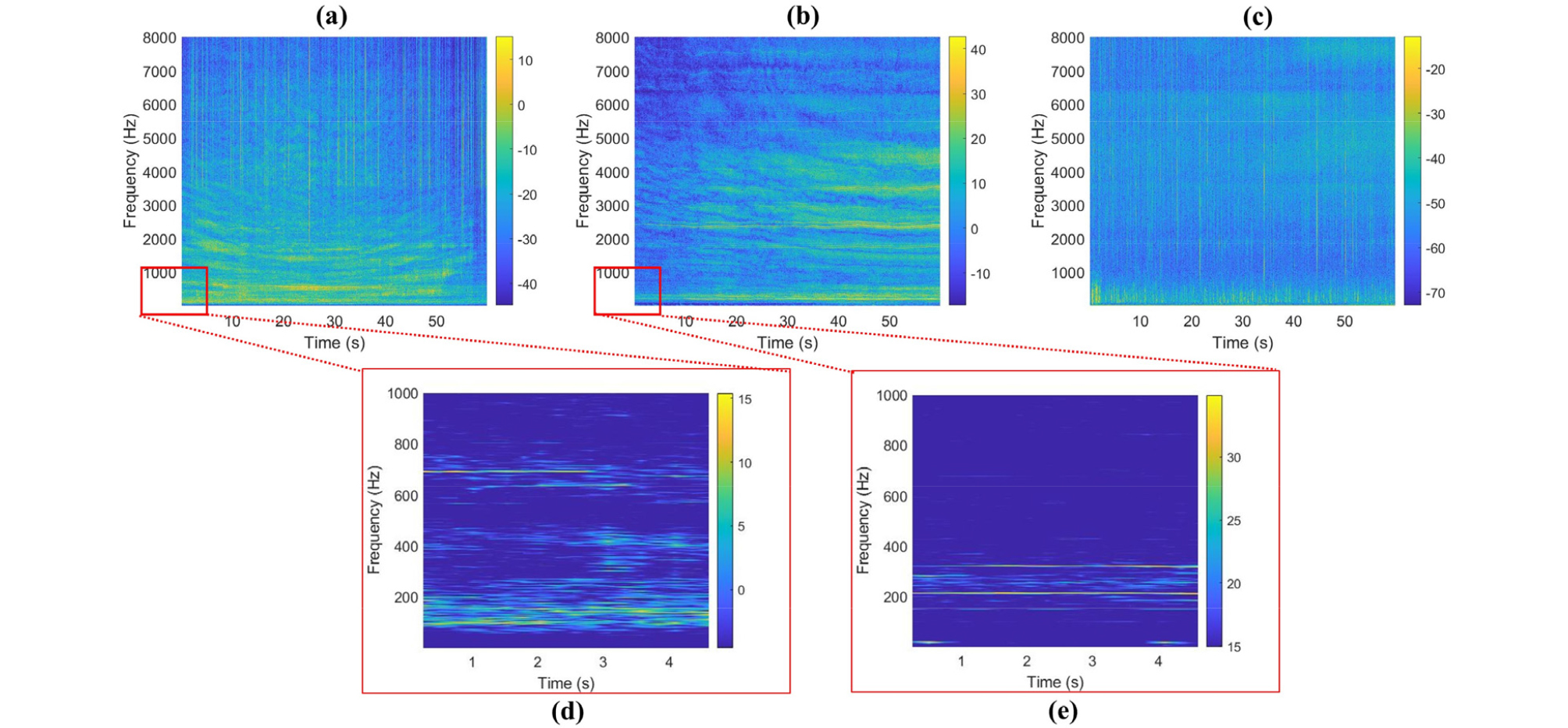
In most cases, basic discrimination of different underwater vessel sounds lie below 1000 Hz and we would be interested in this frequency spectrum. If we look closely at the spectrograms of motorboat and passengerboat as shown in Fig. 1(d) and Fig. 1(e), we can observe the dominant frequency components of each boat discriminating them from each other. The basic task of CycleGAN is to translate one ship engine dominant frequencies to other ship engine frequencies. We hypothesize that the proposed improved version of CycleGAN can better perform this translation.
III. Network Architecture
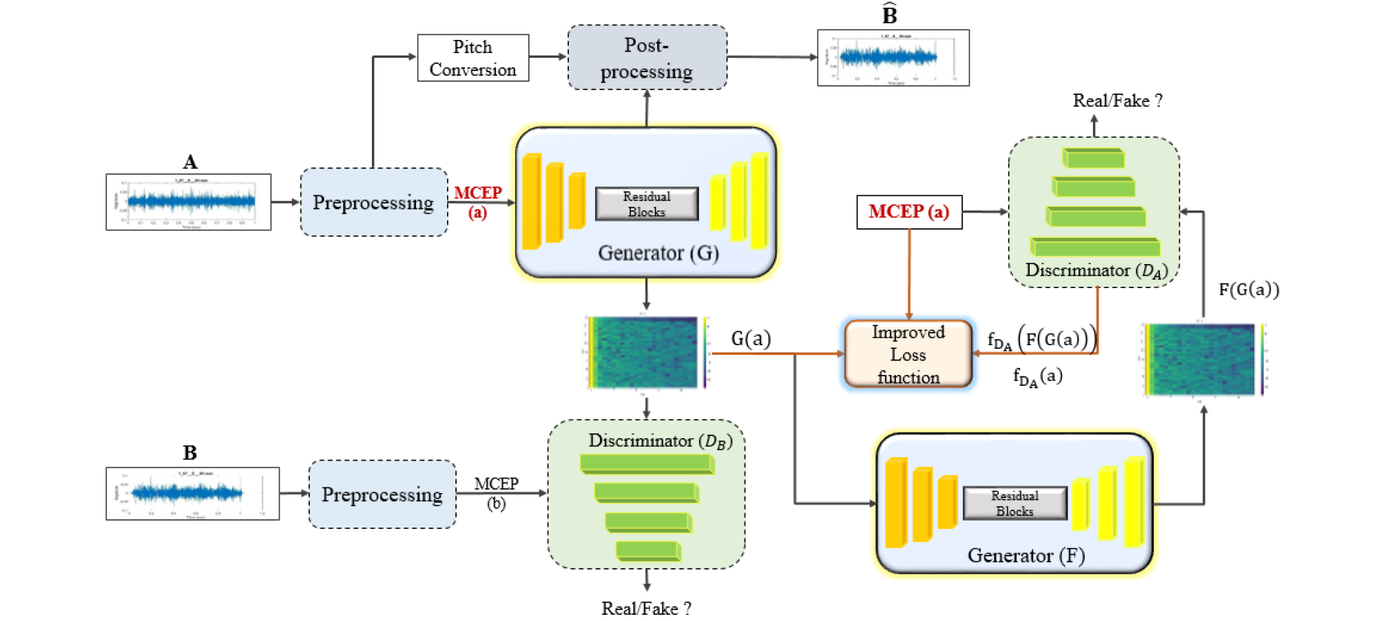
The proposed network adopts network structure of the CycleGAN[21] and achieves improvements by incorporating modified discriminator, a generator with improved up- sampling decoder and a modified objective function. The overall structure of the proposed modified CycleGAN network is shown in Fig. 2.
3.1 Generator Architecture
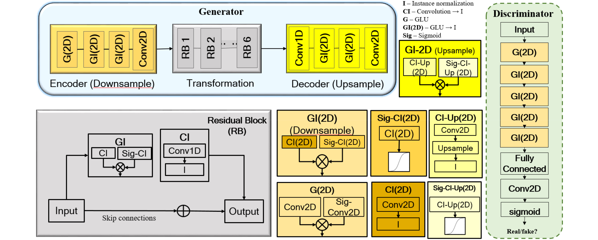
Generator network consist of three major blocks: encoder (down sampling), residual blocks (transformation), decoder (up-sampling). In this architecture, the input is first down-sampled by the encoder network, then it is passed to Residual Blocks (RB) where the stacked multiple convolutional layers, enable building a very deep network to learn feature maps. The output of residual blocks is then passed to decoder block where up-sampling is performed to reconstruct target MCEP as shown in Fig. 3. If CycleGAN is applied straight forwardly to audio-to-audio translations, it needs to first upsample the low-resolution input to the high-resolution by performing interpolation, which also enlarge the noisy patterns. Hence, the direct application of existing CycleGAN causes amplified noise and training also becomes unstable. In previous technique, up-sampling has been done using simple nearest neighbor convolution, which has low performance and introduces noise and checkerboard affect. Instead of using simple up-sampling convolutions, we are using bi-cubic interpolation in generator decoder block, which removes the above-mentioned shortcomings. Gated linear unit in 2-Dimensions (G-2D) block consist of Gated Linear Units (GLUs) where 2D means the input is 2D matrix, which achieved competitive results in signal modeling as LSTM while reducing the computational cost to manifolds. Gated Instance normalized (GI-2D) makes use of instance normalization, which is used for the style- transfer after G-2D block. The last conv2D layer is used to convert two-dimensional matrix into one-dimensional to feed into one-dimensional RB network.
3.2 Discriminator Architecture
Regular GAN discriminator has a global discriminator architecture that observes the whole input at once signifying as real or fake whereas PatchGAN[27] maps from complete input to every partial patches of the input. This way receptive field can be traced back to see which patch or input samples is it sensitive to. In patch-based approach, the generator converges quickly due to operating on each local patch independently. However, attentiveness of the network to view the global spatial information is limited, which in turn limits the ability of the generator to perform coherent audio translation. As a remedy to the problem, the idea is to perform segmentation using dilated convolutions. Dilated convolution requires a lot lesser parameters than required by conventional convolutional networks while maintaining the accuracy. It spreads out the convolution weights to over a wider area to expand the receptive field size significantly, which helps in prediction from larger surroundings and well narrate the dependency between the distant regions. This allows increased information flow between generator and discriminator as the generator knows now which patch or region to focus on.
3.3 Loss Function
With CycleGAN, there is a translator G : A → B and additional inverse translator, F : B → A both with bijective mappings. Both the mappings, G and F are trained simultaneously and a cycle consistency loss is added to encourage F(G(A)) ≈ a and G(F(b)) ≈ b. DB and DA are the associated adversarial discriminators.
Adversarial loss: We apply adversarial losses to both mapping functions. For the mapping function G: A → B and its discriminator DB, we express the objective as,
Similarly, the mapping function for F: B → A and its discriminator DA can be expressed as,
Proposed consistency loss: Since the adversarial loss only restricts to follow the target distribution and does not guarantee audio consistency between the target and source features, consistency loss is introduced. Because cycle consistency encourages generators to avoid unnecessary changes and thus to generate images that share structural similarity with inputs, it can also be viewed as a form of regularization. By enforcing cycle consistency, CycleGAN framework prevents generators from excessive hallucinations and mode collapse, both of which will cause unnecessary loss of information and thus increase in cycle consistency loss. The cycle consistency loss of the original CycleGAN is,
The cycle consistency sometimes causes undesired results since it assumes no information loss during translation even when moderate loss is necessary as in underwater sound domain. To handle this problem, we adopt a weight, α in cycle consistency loss. The weight α starts with small number and gradually increases to a high value close but not equal to 1 to maintain some fraction of pixel level consistency and not to have unwanted results. This helps stabilizing training in early stages but in later stages becomes an obstacle towards realistic results.[30] The final cycle consistency loss is,
| (5) |
where is the feature extractor of the last layer of D(.) and α ∊[0,1]
Similarity mapping loss: For encouraging input preservation, we use similarity mapping loss,
The final loss of the proposed network can be expressed sum of all three discussed losses as follows:
where λcyc and λsim are trade-off parameters between similarity and cyclic losses.
IV. Results
4.1 Dataset
We used ShipsEar,[31] a publicly available underwater dataset for the verification and analysis of results. From this dataset, we have taken two vessel types (motorboat and passengerboat) and ambient noise recordings. The audio recordings have a sampling rate of 52734 Hz. We resampled the audio files at 16 kHz since frequencies of interest for the underwater data lies between 0 to 8000 Hz ranges. The audio recordings are sliced into 5-second chunks of equal length. The dataset from each category contains 133 training examples. For extraction of features, the sampled audio chunks are fed to preprocessing block, where MCEP envelope, logarithmic fundamental frequency () and aperiodicities (APs) are extracted every 5ms within 20ms window using WORLD analyzer. The CycleGAN approach is used to model 24-dimensional MCEPs with 128 time frames. The order of MCEPs can be different for different datasets. In Fig. 4, we have plotted the loss curves for different number of MCEPs, which shows the network performance is almost similar if MCEPs are chosen to be 24 or 34. We have taken the number of coefficients to be 24, since it is computationally efficient while maintaining the network performance.

For simulation parameters, we have used least square loss function to calculate the adversarial loss since it results in stable training and higher quality audios. Adam optimizer with a batch size of 2 is used as an adaptive learning rate optimization algorithm. At start, the learning rates of the generator and the discriminator are set to 0.0002 and 0.0001, respectively. For each epoch, it decayed by 2 × 10⁵. The trade-off parameters λcyc is set to 10 and λsim is set to 1 for the initial 100 epochs and then to zero after 100 epochs.
4.2 Spectral Feature Representation Analysis
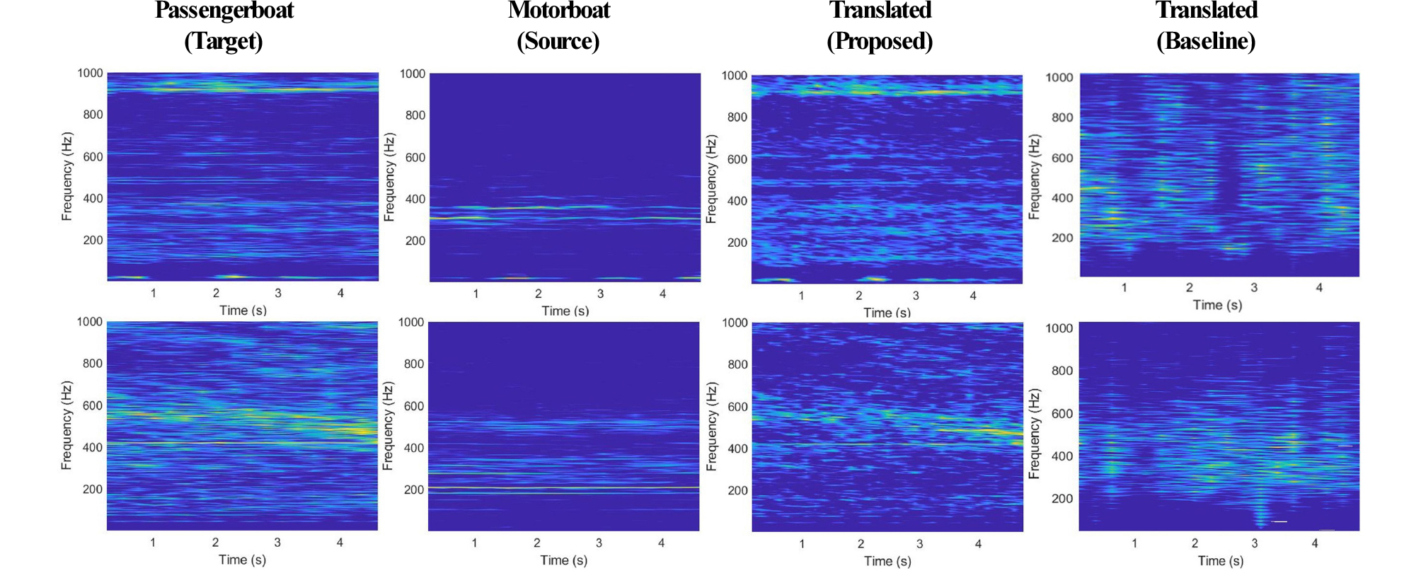
To evaluate the performance of the proposed algorithm, we conduct the experiment of engine sound style change from motorboat to passengerboat. The spectrogram outputs of source, target and style changed outputs are shown in Fig. 5. We can observe that the frequency components of the target audios are present in translated audios by the proposed algorithm. In first row of Fig. 5, the few dominant frequency components are around 200 Hz and 900 Hz for target passengerboat while for motorboat it lies around 300 Hz and 150 Hz. In translated spectrogram, one can observe the frequency component present around 200 Hz and 900 Hz while in baseline translated spectrogram, it is mostly closer to source Motorboat. The translated spectrograms by baseline CycleGAN also have increased noise as compared to the proposed technique due to the upsampling layer. Looking at these examples, we can say that the proposed CycleGAN has successfully changed source sound to target sound while the original CycleGAN fails in sound style change.
4.3 Analysis
4.3.1 Quantitative Analysis
To quantify total structural differences, we took the Mel-cepstral distortion (MCD)[32] parameter, which calculates the distance between the target and converted MCEP structures. This quantity is measured using Eq. (8), a smaller value indicates that the target and converted MCEPs matches with each other. The results of the MCD is listed in Table 1.
where , and D are the ith MCEP coefficient of the target and converted audios and D is the order of MCEP features, respectively. Another measure to assess the output MCEPs with the target MCEP is chosen as Structural SIMilarity (SSIM).[33] The value of this parameter ranges between 1 and –1, where 1 shows the two images as identical. The SSIM can be calculated as follows:
Table 1.
Qualitative and quantitative comparison with other techniques for motorboat audios.
| No. | Methods | MCD [dB] | MOS [0-5] | Nearest neighbor (Dist) | Mode collapse |
| 1 | WaveGAN [11] | 9.37 | 3.01 | 0.38 | ✔ |
| 2 | Baseline CycleGAN [20] | 8.05 | 3.1 | 0.32 | ✖ |
| 3 | Proposed CycleGAN (Our) | 6.86 | 3.6 | 0.29 | ✖ |
where μm, μn, σm, σn, and σmn are the local means, standard deviations, and cross-covariance for images m, n. The training error plots for the measure SSIM and Mean Square Error (MSE) are shown in the Fig. 6, in which we can observed that the proposed network relatively low training error than original CycleGAN for the translation of motorboat engine audios to passengerboat audios (mo- pa).
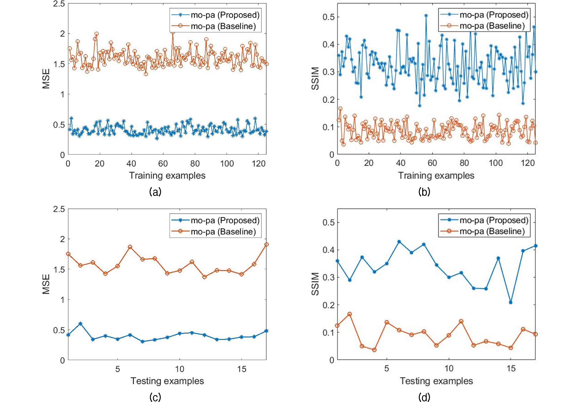
Fig. 6.
(Color available online) Comparison plots for translation from motorboat to passengerboat for the baseline and modified CycleGAN. (a) MSE comparison plot for training dataset, (b) SSIM comparison plot for training datasets, (c) MSE comparison plot for testing datasets, (d) SSIM comparison plot for testing datasets.
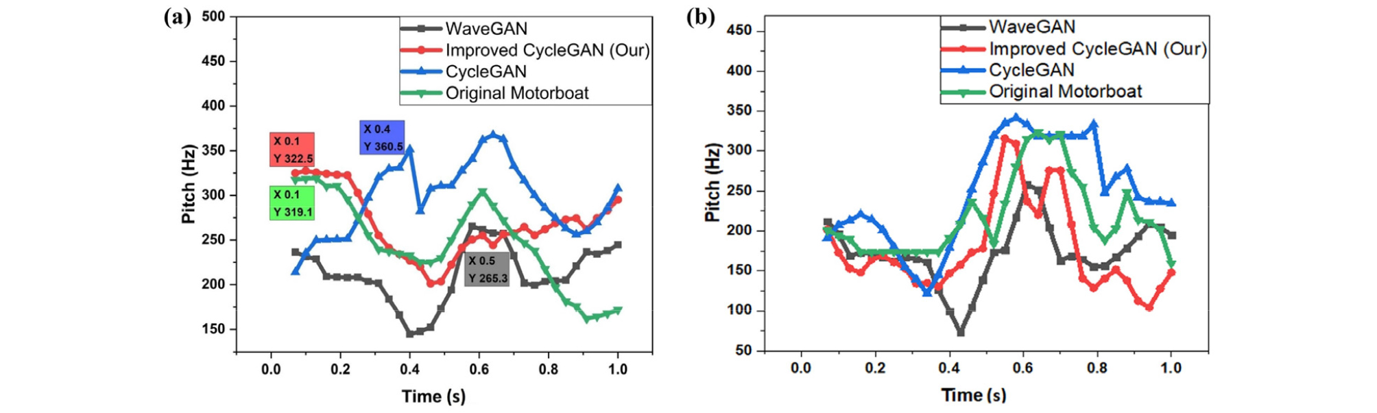
As a second metric to compare the generated underwater audios with the original audios, we have chosen pitch contours that focus on the relative change in pitch over time. The fundamental frequency is estimated for each frame by segmenting the audio input according to a given window length and overlap. We are using Pitch Estimation Filter (PEF) to estimate fundamental frequency contours of translated and original audios by using window length set to 70 ms and with an overlap of 40 ms. The pitch contours of other algorithms are shown in the Fig. 7 after style transfer from ambient noise to motorboat and passengerboat to motorboat. Notice that the proposed algorithm follows the pitch contours of the original audio better than the baseline CycleGAN and WaveGAN.
To calculate distances in the frequency-domain, we use test dataset consisted of 17 underwater motorboat samples given to the presented trained model and translated to passengerboat sounds. The ‘Dist’ represents the average Euclidean distance between 133 training samples and 17 generated samples from the test dataset. A low value justifies the similarity, if the generated examples are from the training dataset, its value will be 0. The audio generated with the proposed CycleGAN does not suffer from mode collapse problem in which generator model produces limited varieties of samples. Unlike WaveGAN, the cycle consistency loss of CycleGAN ensures that the generative model does not incur mode collapse. The performance superiority of the improved CycleGAN with other techniques in terms of above explained metrics is summarized in Table 1.
4.3.2 Qualitative Analysis
We have chosen MOS[34] as the measure of quality of the generated audios with respect to original audios. Our ultimate goal is to produce ship engine audio examples that are recognizable to humans. To this end, we measure the ability of human annotators to label the generated audio either from the motorboat or passengerboat category. We translate 17 examples from testing data and ask annotators to label which category they perceive in each example, and compute their score with respect to the actual labels. Annotators assign subjective values of 1-5 (1 being poor and 5 being excellent) for the criteria of sound quality and a classification category (motorboat and passengerboat). The value MOS can be calculated by using the following Eq. (10).
| $$\mathrm{MOS}=\frac{\sum_{i=1}^NR_{\mathrm i}}N,$$ | (10) |
where N are total human subjects and R is the assigned individual ratings.
To measure the similarity in terms of listening audios, we calculated average accuracy of the correctly recognized audios from two categories. We report accuracy (n = 17) and MOS in the following Table 2. We can observe that the proposed network is superior to original CycleGAN for all style transfers.
Table 2.
Comparison of the improved CycleGAN with baseline CycleGAN technique.
V. Conclusions
We proposed a modified version of CycleGAN for transfer of underwater ship engine sound to another style sound. The proposed algorithm is composed of modified generator, modified discriminator and improved cycle- consistency loss function. The audio results generated are quantified using various performance metrics, which include Mel-cepstral distortion, structural similarity, pitch contours, nearest neighbor and mean opinion score. The experimental results of using underwater audio dataset, demonstrate that the proposed algorithm outperforms original CycleGAN and other audio style transfer networks in both quantitative and qualitative measures of the generated sounds.
